A tutorial on implementing and interpreting LocalGLMnet using PyTorch and Python

At Eika Forsikring we believe that there is a lot to be gained by expanding the actuarial toolkit with techniques that are most commonly used within the field of data science. This is why our pricing actuaries and data scientists work closely together on a variety of problems within the actuarial space. In this blog post we will take a closer look at how we’ve approached the issue of variable selection when the number of variables is too large to be assessed using conventional methods. While attending the Insurance Data Science conference in Milan in 2022 we became familiar with a neural network architecture known as the LocalGLMNet (Richman, 2021) that offered a new and exciting way of approaching this problem. By inspecting the weights of the attention layer in this neural network it is possible to understand which variables the neural network has identified as having a meaningful impact on our response variable. It is even possible, with some additional work, to understand how variables interact with each other in the network.

Although the idea behind the LocalGLMNet is interesting on its own, we will not provide a full treatment here, seeing it has already been very well covered in [Richman, 2021] and [Schelldorfer, 2021]. The focus here will rather be on the implementation in Python — more specifically, how the neural network can be set up and trained in PyTorch and how insights about the behavior of the network can be obtained. In the following we therefore only provide a short overview of the idea behind the LocalGLMNet.

An overview of LocalGLMNet

The core idea behind the LocalGLMNet is to create a generalized linear model, GLM for short, where the coefficients, $\mathbf{\hat{\beta}}$, are functions of the input variable $\mathbf{x}$. An evaluated “coefficient function” will be referred to as an attention.

$$ \hat{Y} = g^{-1}\left(\hat{\beta_0} + \sum_{i=1}^p\hat{\beta_i}\left(\mathbf{x}\right)x_i\right) $$

By extracting the attentions, $\hat{\beta_i}(\mathbf{x})$, from the neural network, we can obtain insights about the importance of the different variables. An attention that remains close to zero regardless of the value of the input tells us that the corresponding variable is of little importance when trying to explain the behavior of our response. One can also plot the product of the variable values and the attentions, $\mathbf{\hat{\beta}}_i(\mathbf{x})x_i$, from now on referred to as contributions, in order to better understand how each variable impacts the response.

The gradients of the various attentions with respect to the different variables, $\frac{\partial\hat{\beta}_j(\mathbf{x})}{\partial x_k}$, are also of interest. These can tell us how the attention of one variable interacts with another variable within the network.

Interpretation of the attentions require that all the variables live on the same scale. It is therefore necessary to standardize the continuous variables so that all have mean zero and unit variance. A similar treatment does not make sense for categorical variables, and the insight into behavior of the categorical variable is therefore not as extensive as what we obtain for the continuous variables.

Because there are no theoretical results available about exactly how the attentions of a variable that is unrelated to the response should behave, it is useful to include a random feature in our data. This provides us with what we need for conducting an empirical hypothesis test of the importance of our other variables. The idea is that if the attentions of a variable often are larger than the attentions associated with the random feature one can conclude that the response has some dependence on the variable.

LocalGLMNet in PyTorch

For the purpose of demonstration we use the openly available insurance dataset known as freMTPL2freq. It can be downloaded from OpenML. This dataset contains risk features for motor third-party liability policies as well as the number of claims and the exposure of each of the policies. The file available from OpenML is an ARFF file. It can be converted to a Parquet file in R using foreign::read.arff and arrow::write_parquet.

Preprocessing

We start off by loading our data and splitting it into a train set and a test set. This is followed by the creation of a preprocessing step that standardizes the numerical variables and one-hot encodes the categorical variables before applying it to the data.

import pandas as pd
import numpy as np
from sklearn.compose import ColumnTransformer
from sklearn.preprocessing import StandardScaler, OneHotEncoder
from sklearn.model_selection import train_test_split

data = pd.read_parquet("freMTPL2freq.parquet")

response_variable = "ClaimNb"
exposure_variable = "Exposure"
categorical_variables = ["Area", "VehBrand", "VehGas", "Region"]
continuous_variables = ["DrivAge", "Density", "VehPower", "BonusMalus", "VehAge"]

data = (
    data
    .drop(columns=["IDpol"])
    .assign(
        **{c: lambda x, c=c: x[c].astype("category") for c in categorical_variables},
        **{
            c: lambda x, c=c: x[c].astype("float32")
            for c in [*continuous_variables, response_variable, exposure_variable]
        },
        RandN=lambda x: np.random.normal(size=x.shape[0])
    )
)

y = data[[response_variable]].to_numpy()
v = data[[exposure_variable]].to_numpy()
X = data.drop(columns=[response_variable, exposure_variable])

X, X_val, v, v_val, y, y_val = train_test_split(X, v, y)

transformer = ColumnTransformer(
    [
        ("continuous_pipeline", StandardScaler(), continuous_variables),
        (
            "categorical_pipeline",
            OneHotEncoder(sparse_output=False),
            categorical_variables,
        ),
    ],
    remainder="passthrough",
    sparse_threshold=0,
    verbose_feature_names_out=False,
)

X = transformer.fit_transform(X).astype("float32")
X_val = transformer.transform(X_val).astype("float32")

Defining the neural network

Now that we’ve transformed our data we can move on to setting up our neural network.The following contains the implementation of LocalGLMNet as a PyTorch module. It closely follows the Keras implementation in R included in the appendix of [Richman, 2021], but uses the log link instead of the identity link, and also adds support for including an exposure variable.

import torch
from torch import nn
from torch.optim import NAdam


class LocalGLMNet(nn.Module):
    def __init__(self, input_size, hidden_layer_sizes):
        super(LocalGLMNet, self).__init__()

        self.hidden_layers = nn.ModuleList(
            [nn.Linear(input_size, hidden_layer_sizes[0])]
        )
        self.hidden_layers.extend(
            [
                nn.Linear(hidden_layer_sizes[i], hidden_layer_sizes[i + 1])
                for i in range(len(hidden_layer_sizes) - 1)
            ]
        )
        self.last_hidden_layer = nn.Linear(hidden_layer_sizes[-1], input_size)
        self.output_layer = nn.Linear(1, 1)
        self.activation = nn.Tanh()
        self.inverse_link = torch.exp

    def forward(self, features, exposure=None, attentions=False):
        x = features
        for layer in self.hidden_layers:
            x = self.activation(layer(x))
        x = self.last_hidden_layer(x)
        if attentions:
            return x
        # Dot product
        skip_connection = torch.einsum("ij,ij->i", x, features).unsqueeze(1)
        x = self.output_layer(skip_connection)
        x = self.inverse_link(x)
        if exposure is None:
            exposure = torch.ones_like(x, device=features.device)
        x = x * exposure
        return x

Training the neural network

The next step is to train our neural network. We leverage the Python library skorch for this purpose, seeing as this removes a considerable amount of boilerplate code that is typically needed when training a neural network in PyTorch. When setting up NeuralNetRegressor we must choose which loss function to minimize. Since we’re in the business of frequency modeling it makes sense to go with PoissonNLLLoss.

Before training the network we also need to make choices with regards to the number of layers and hidden units, batch size, number of epochs and learning rate. It might be sensible to do some sort of hyperparameter search to identify the optimal value of these, but we choose not explore this any further here.

When this is done all we have to do is call the fit method.

from skorch import NeuralNetRegressor

localglmnet = NeuralNetRegressor(
    module=LocalGLMNet,
    max_epochs=10,
    criterion=nn.PoissonNLLLoss,
    criterion__log_input=False,
    module__input_size=X.shape[1],
    module__hidden_layer_sizes=[64, 32, 16],
    optimizer=NAdam,
    lr=0.01,
    batch_size=512,
    device="cuda",
)

X_dict = {"features": X, "exposure": v}
localglmnet.fit(X_dict, y)

Extracting attentions and contributions

Now that we have trained the LocalGLMNet we want to learn about the patterns it has identified in our data. We get the attentions instead of the prediction by passing attentions = True to the forward method of our PyTorch module. Since the LocalGLMNet has an output layer that scales and shifts the output of the dot layer we must multiply our attentions with the weight of the output layer to obtain attentions that are on the right scale. Contributions are obtained by simply multiplying the attentions with their corresponding feature value.

localglmnet_module = localglmnet.module_.to("cpu")
unscaled_attentions = localglmnet_module(
    torch.from_numpy(X_val), exposure=v_val, attentions=True
).numpy(force=True)
scaling = localglmnet_module.output_layer.weight.numpy(force=True)
attentions = unscaled_attentions * scaling
contributions = np.multiply(attentions, X_val)

Attentions

The attentions are visualized in the following figures. The blue lines show lower and upper bound of our empirical confidence interval, which covers 99.9% of the “random attentions”. Variables that frequently have attentions outside these regions is assigned at least some importance by the LocalGLMNet.

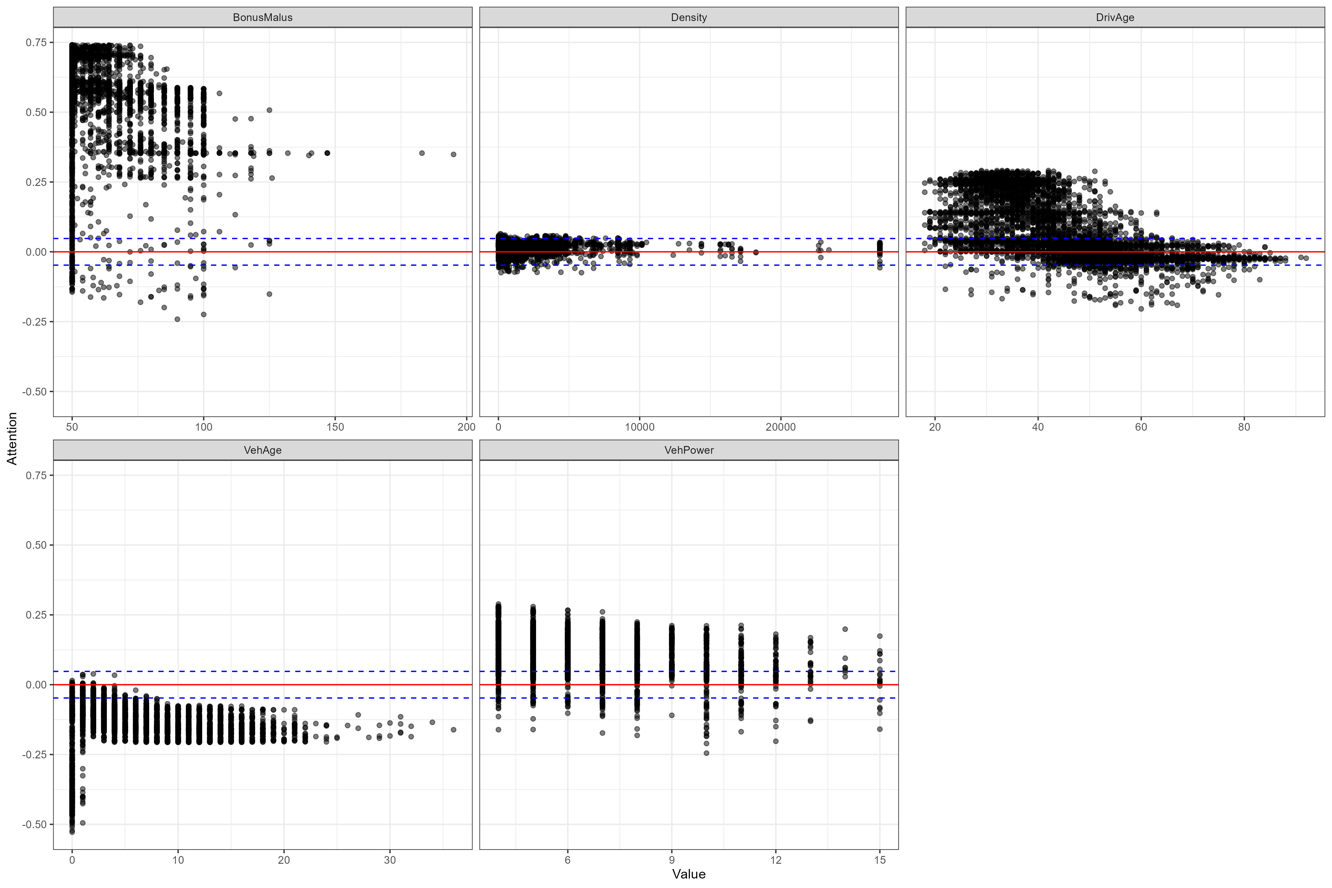
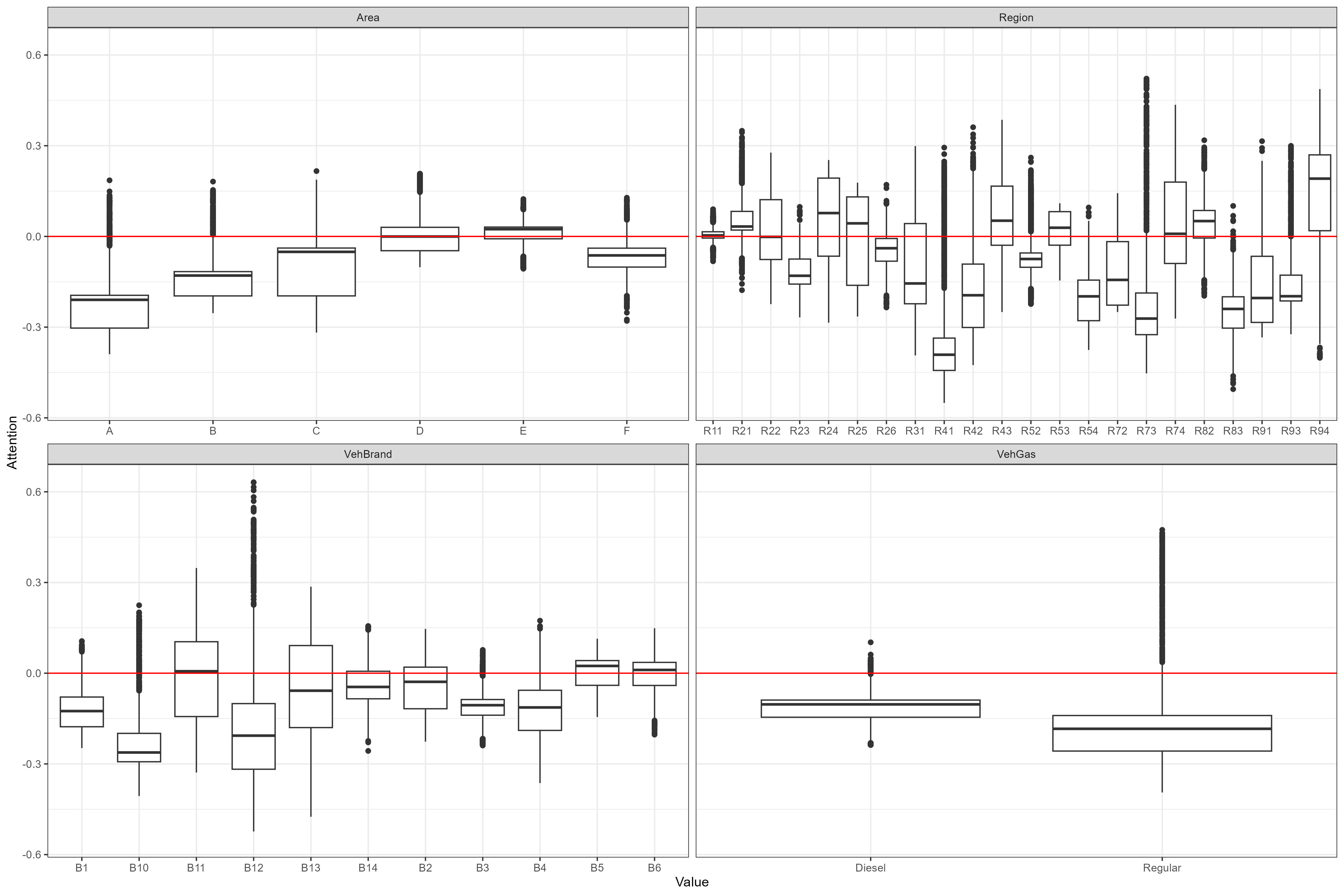
Confidence intervals are not available for categorical attentions, but the distribution can differ considerably between levels, which indicates that the information is utilized by the neural network to some extent. High variation within a level indicates a larger degree of interaction with other variables.

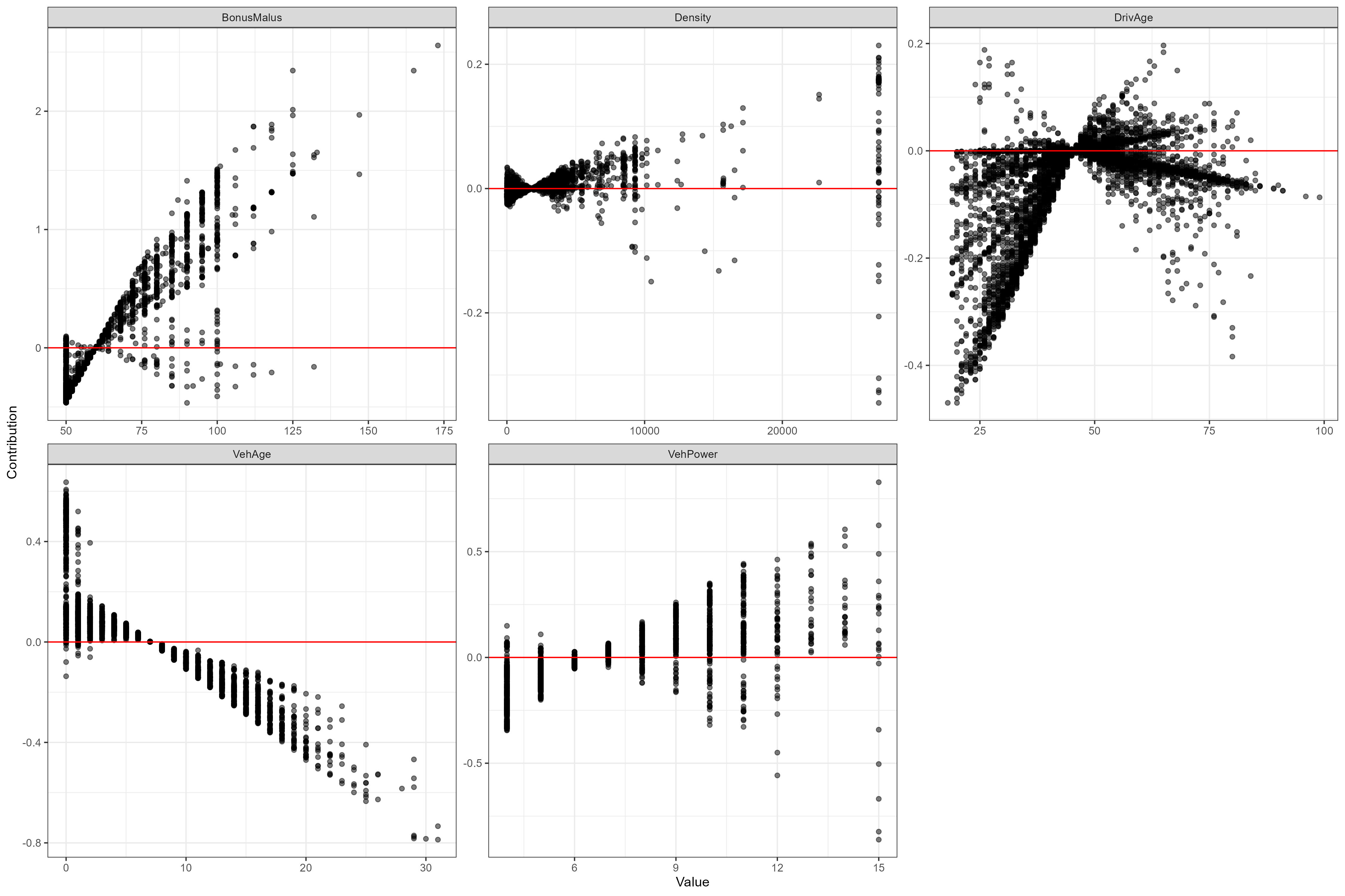
Contributions

By multiplying the attentions with their corresponding feature value we can see the relationship between the variable and the response. Note that there isn’t much point in doing this for the categorical variables, seeing as these are one-hot encoded.

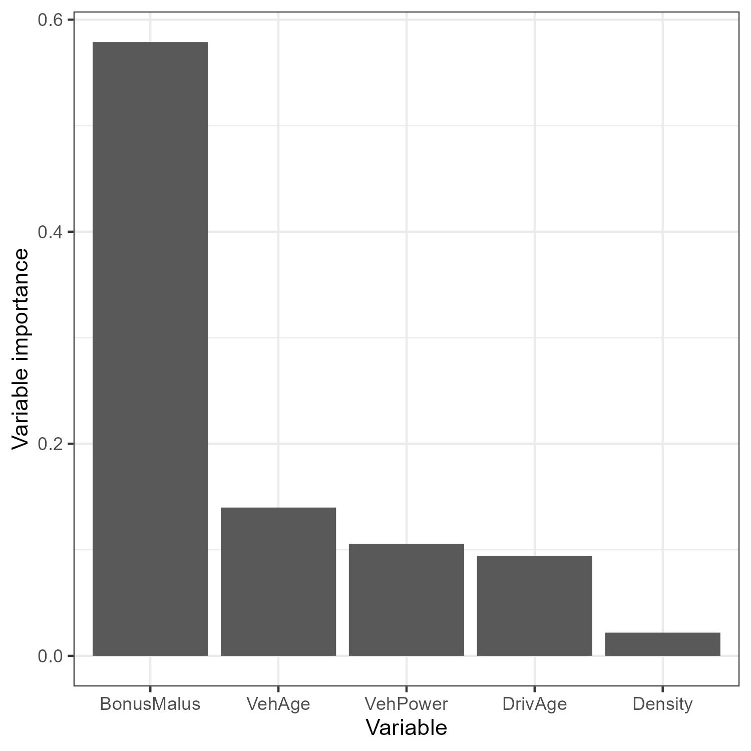
Variable importance

By taking the mean absolute value of the attentions we obtain something that can be thought of as variable importance.

Extracting the gradients

The final thing we’re going to look at are the interactions that the network has identified, which we can learn about by looking at the gradients of the attentions. The following code shows us how we can obtain these gradients for our data.

import torch.autograd as autograd

input_tensor = torch.from_numpy(X_val)
input_tensor.requires_grad = True
attentions = localglmnet_module(input_tensor, exposure=v_val, attentions=True)

n, p = input_tensor.shape
gradients = np.empty((p, n, p))
for i in range(p):
    grad_scaling = torch.ones_like(attentions[:, i])
    gradient_i = autograd.grad(
        attentions[:, i], input_tensor, grad_scaling, create_graph=True
    )
    gradients[i, :, :] = gradient_i[0].numpy(force=True) * scaling

Interactions

The gradients show us how the attentions change as the feature values are varied. The figures show a spline that has been fit to the extracted gradients. In each plot we the see the gradient of a specific attention component as all the other (numerical) variables are varied. We will not delve any deeper into the interpretation of the gradients, but anyone interested in this should take a look at the original LocalGLMNet paper (Richman, 2021).

Closing remarks

I hope this short overview of LocalGLMNet, its implementation and its use can be of interest to people who are exploring how to leverage cutting-edge techniques and technologies in actuarial applications without losing track of how the model behaves. At Eika Forsikring we’ll be sure to keep engaging with this topic, and there might even be another blog post coming if we stumble across something particularly interesting!